Introduction 

In the quest for accurate and efficient signal estimation in the digital signal processing (DSP), Kalman filters have emerged as a powerful tool for filtering and predicting the state of dynamic systems. Originally developed for applications in aerospace and navigation, Kalman filters have found their way into many fields, from finance to robotics. 

In this blog, we delve into the fundamentals of Kalman filters, explore the need for adaptation, and discuss how adaptive Kalman filters enhance the performance of different DSP applications. Whether you are a seasoned engineer or a curious enthusiast, this guide will provide a better understanding of this fascinating topic. 

What is a Kalman Filter? 

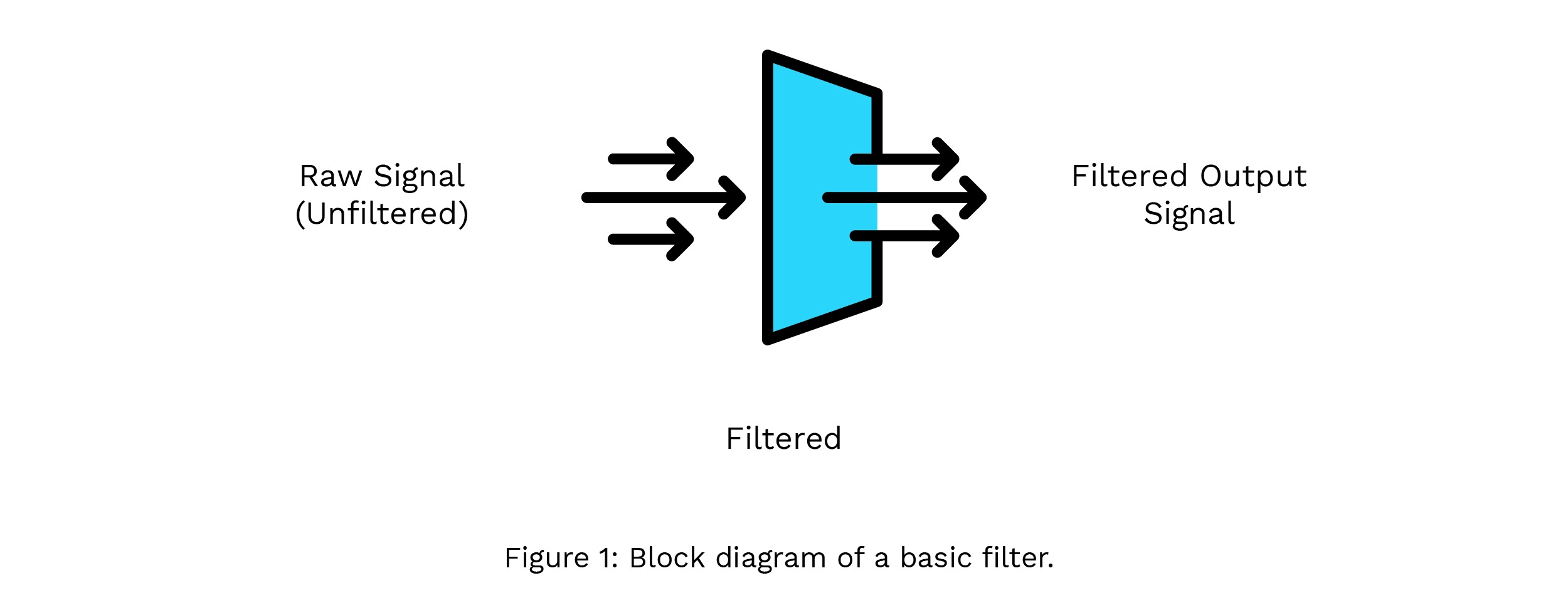
Before understanding Kalman filters, let us briefly understand what a “filter” traditionally means. In signal processing, the role of a filter is to remove unwanted parts of the signal while extracting the useful parts of the signal. These filters can be of two types – analog, which are analog electronic circuits based on resistors, capacitors, and inductors, and digital, which use a digital processor and mathematical equations on a digitally acquired signal. 

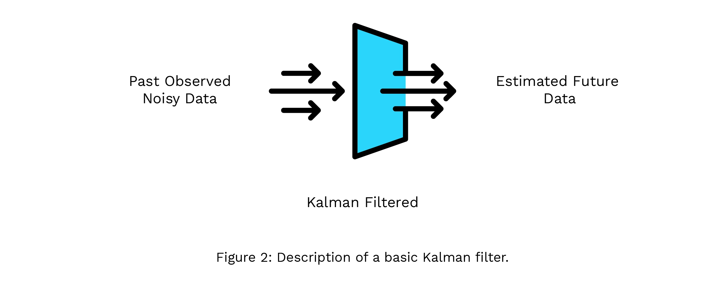
Kalman filtering, in a nutshell, takes in a series of measurements observed over time and produces an estimate of the next value based on the previously observed values. The filter is named after Rudolf E. Kálmán, who was one of the primary developers of its theory. 

If you feel that the above description for Kalman filters does not seem to fit the traditional definition of a filter above, you are right. The fundamental focus of a Kalman filter is to optimally estimate the future data from an existing data set from the past. A Kalman filter is a “smart guesser”. However, if we take a closer look at the input series of measurements itself it is likely that these sets of data will include deviations, or noise, that the filter will need to go through to optimally “guess” the future data. Hence, by adding noise to the input data, we see that a Kalman filter starts to better fit the traditional definition of a digital filter as we described above.  

How Does the Filter Work? 

While there are mathematical equations to help answer that more precisely, we will restrict ourselves here to building a more intuitive understanding of the filter with a real-life application of GPS navigation and tracking. 

Let us imagine you are on a road trip, and you are using a GPS application on your phone to track your real-time location. The application uses data from the satellites to estimate your position, but this data can be noisy or inaccurate. The application uses a Kalman filtering to smooth out these inaccuracies and give you a relatively accurate idea of your position on the map. 

The standard Kalman filter algorithm cycles through three basic stages: Measurement, Prediction and Update (Figure 3). 

1. Measurement Stage: The actual readings are taken in this stage. We can also include the stage of Initialization in this, where some parameters of the filters are set to their default values. 

In the example of GPS navigation, this stage is where the noisy GPS readings are taken in by the phone’s GPS sensor and read by the application. Some parameters like your initial speeds, direction and the errors of that initial position are also noted by the filter. 

 2. Prediction Stage: Based on the parameters of the filter and the measurements taken in previous stage, this stage of the filter predicts the next state of the system. 

This stage is where the GPS application tries to guess where your car will be in the next second based on your previous speeds and direction, even before you have travelled that distance. 

This stage is also the cause behind many popular navigation applications today sometimes assuming that you are still travelling the highlighted path for a few seconds until the application realizes you have taken a different turn and rerouting to that path. 

 3.Update Stage: The filter then takes in the predicted value and the noisy measurements and weighs them based on how much “uncertainty” they carry. The new result is updated on the map and is more accurate than either the prediction or the measurement. This “uncertainty” value is dictated by the Kalman Gain of the filter. 

In our example, this stage is where the GPS application combines your predicted position and the GPS data to update your next position. If the GPS data is accurate, the application trusts it more and increases the Kalman Gain. However, if the prediction model seems more accurate, the application trusts that instead and consequently decreases the Kalman Gain. 

Why the Necessity for Adaptation? 

Among the three stages of the Kalman filter, the emphasis is on the change in the useful GPS data from one point of time to the next.  

So, what if the noise itself within the GPS data changes?  

The major drawback of the standard Kalman filter is that it assumes the noise within the measured data from the Measurement Stage is consistent and known. This is rarely the case in the real world as noise is inherently highly dynamic and can change rapidly in short periods of time. This can corrupt the measured data significantly differently each time it is taken. 

This is where the Adaptive Kalman Filter comes in and gives the standard Kalman Filter the ability to learn and adjust its settings on the fly. When it notices that you have started moving faster or that the GPS signal quality has changed, it adapts its calculations to better handle these new conditions. This way, it can continue to provide accurate location estimates even when things change unexpectedly. 

Adaptive Kalman filters use a few different techniques in the Update Stage to not only update the Kalman Gain, but also the noise models in the measurements taken in the first Measurement Stage itself. This allows the Prediction Stage to refer to this data and make a better prediction of the future state. These techniques constantly evolve with ongoing research. 

How does the Filter Adapt? 

To understand how the filter adapts using different techniques, we need to first understand the two types of noises that are extracted out from our GPS signal – measurement noise and process noise.  

1. Measurement Noise: The GPS sensors are developed and designed to work in a specific set of conditions. If any deviations are observed from these conditions, there can occasionally be errors in data captured by the GPS data. Measurement noise covers only errors caused by the inherent inaccuracies and limitations of the sensors.  

One way to detect and reduce this noise is by adding more sensors to the array which would add redundancy while covering the inaccuracies caused by the other sensors. 

 2. Process Noise: When the GPS sensor travels from a clear sky to a cloudy sky or through a tunnel, there is a visible drop in accuracy of the GPS data. Process Noise covers only those noises caused by changes in the sensor’s environment. 

The adaptive techniques of Kalman filters primarily focus on adapting to this type of noise. 

Let us go back to our example of the GPS application. To have a robust Update Stage for updating its parameters, the filter needs to understand how well it has predicted the next state in the Predict Stage. One way to do this is by taking the difference between the predicted value and the measured value from the Measurement Stage. Let us refer to this difference as the error in the predicted value (Figure 4). This gives us the following three conditions. 

• Normal Noise Conditions:  

• • The filter compares the measured readings with the predicted values.  

• • Since the error would be under limits, no adjustments are needed in the extracted Process Noise for the next iteration of the algorithm.  

• • This, in turn, increases the Kalman Gain which increases the validity of the GPS sensor data. 

• Increasing Noise Conditions: 

• • Suddenly the GPS signal starts giving less reliable measurements. 

• • Error values start becoming larger than expected which is detected by the filter. It starts to automatically adjust the values of the extracted process noise detected in the signal based on these increased error values. 

• • This leads to a decrease in Kalman Gain, increasing the weightage given to the Kalman predicted data instead of the GPS sensor data. 

• Decreasing Noise Conditions: 

• • GPS signal starts to improve the measurements and starts becoming stable. 

• • Error values reduce and reach the lower limits again which triggers the filter to readjust the process noise values based on the decreasing error values. 

• • The filter starts increasing the Kalman Gain again and the weightage is given again to the GPS sensor data. 

This adaptation strategy is also referred to as the Innovation-Based Adaptation algorithm for an Adaptive Kalman filter, where the term “Innovation” is the error calculated from the difference between the predicted and the measured values by the Kalman filter. 

Other Applications of the Kalman Filter 

We have looked at one of the applications, on-road vehicular navigation, and positioning system, where the Adaptive Kalman filters are currently used. However, Adaptive Kalman filters are like the Swiss Army knives of the signal processing filters. Dynamically adjusting to changing conditions and uncertainties, these filters are being used in a lot of different domains and have become quite ubiquitous in their usage. 

• Autonomous Vehicles: Imagine self-driving cars navigating through foggy streets. Adaptive Kalman filters help these vehicles stay on track by continuously tweaking their sensor data, ensuring safe and accurate navigation. 

• Robotics: In the world of robotics, these adaptive algorithms enable robots to adapt to ever-changing environments, making them better at mapping, navigating, and performing tasks autonomously. 

• Finance: Stock markets are notoriously unpredictable. These filters, better known in the statistics world as Linear Quadratic Estimation (LQE) algorithms, step in to provide traders with more reliable asset value estimates, adapting to the market’s mood swings and helping make smarter investment decisions. 

• Environmental Monitoring: Adaptive Kalman filters become the guardians of our planet by enhancing environmental monitoring systems, ensuring accurate tracking of air quality, temperature, and pollution levels, even when sensor reliability fluctuates. 

• Healthcare: In healthcare, Adaptive Kalman filters are lifesavers. Wearable health monitors use them to provide precise readings of vital signs, adapting to varying noise levels and ensuring timely medical interventions. 

• Aerospace: From aircraft to spacecraft, these filters are the navigators. They adjust to different altitudes, speeds, and atmospheric conditions, ensuring precise guidance and control in the vast expanse of the sky and beyond. 

Conclusion 

Adaptive Kalman filters represent a significant leap forward in the realm of state estimation and control. By dynamically adjusting to changing conditions and uncertainties, these filters enhance the accuracy and reliability of systems across various domains. The versatility of Adaptive Kalman filters makes them indispensable in our rapidly evolving technological landscape. 

At eInfochips, as we continue to push the boundaries of innovation, these real-time adaptable technologies will become the key to overcoming new challenges and achieving greater levels of precision and reliability of our products.