Biquad filters are tiny, powerful tools that are used in everything from audio mixing and telecommunications to biomedical signal analysis. Whether it is an equalizer on your mobile device, or a fitness tracker magically smoothing out erratic sensor data, these filters shape today’s signal processing applications in countless different ways.

Traditional explanations of digital filters can often feel abstract, filled with complex equations. But at their core, biquad filters operate on a remarkably simple principle. This article demystifies them by looking at their fundamental “recipe,” helping you to intuitively understand how they transform a stream of numbers step-by-step.

Understanding Biquad Filters

At its heart, a biquad filter is defined by a difference equation. Think of this equation as a recipe or a roadmap that instructs a computer on exactly how to calculate its next output sample (y[n]). It does this by using just a few instructions at each step.

• Current input number (x[n]) – This is the new piece of data or sound sample arriving right at that moment.
• Two past input numbers (x[n−1], x[n−2]) – The filter “remembers”! It keeps track of the data that just arrived a moment or two back.
• Two of its own past output numbers (y[n−1], y[n−2]) – This is where things get interesting; the filter also “remembers” what it produced in the very recent past and uses that too!

A biquad filter is a second order filter, meaning its difference equation represents a second order system. The filter order determines the steepness of the frequency response; higher-order filters, or order filters, have a steeper roll-off. Second order filters like the biquad are commonly used as building blocks, and higher-order filters are often implemented by cascading multiple second order sections, each realized as a biquad filter.

In digital signal processing, the digital biquad filter is a standard building block for implementing stable and efficient second order sections. The filter coefficients (b0, b1, b2, a1, a2) directly determine the filter’s frequency response and stability. The transfer function of a biquad filter describes its behavior in the frequency domain.

Companies like Texas Instruments and Analog Devices have played a significant role in supporting research and development in digital signal processing and biquad filter technology.

Introduction to Digital Signal Processing

Digital signal processing (DSP) is the science and art of analyzing, modifying, and interpreting signals, such as sound, images, and sensor data, using digital technology. At its core, DSP transforms real-world information into digital signals that computers and digital signal processors (DSPs) can understand and manipulate. This process allows for precise control, analysis, and enhancement of data, making it possible to filter noise, extract meaningful features, and optimize the performance of countless systems.

DSP is the backbone of modern signal processing, powering everything from audio and video processing to communications, control systems, and multimedia signal processing. By applying sophisticated algorithms, engineers can process signals in real time, enabling applications like speech recognition, image enhancement, and even advanced artificial intelligence and machine learning models.

Digital signal processors are specialized microchips designed to handle the complex mathematical operations required for processing digital signals efficiently. These processors are found in smartphones, medical devices, automotive systems, and countless other technologies that rely on the rapid and reliable analysis of data.

In essence, digital signal processing is what allows us to convert, analyze, and control signals in the digital domain, unlocking new possibilities for innovation and performance. Within this field, digital filters, such as the biquad filter, play a crucial role in shaping and refining signals to meet the needs of modern applications.

The “roadmap” itself looks like this:

y[n] = b0 * x[n] + b1 * x[n-1] + b2 * x[n-2] – a1 * y[n-1] – a2 * y[n-2] 

This is called a standard form for a biquad filter.

The coefficients b0, b1, b2, a1 and a2 are the filter’s coefficients. These are like the “tuning knobs” or “weights” of the ingredients in our recipe. By changing their values, we can instantly change how much influence the current input, past inputs and past outputs have, thereby completely altering the filter’s behavior.

Input Signal, Memory, and Feedback

To understand what the standard form of the biquad equation means, let us try to build a simple low pass filter visually. We will see how the output signal reacts to the feed-forward and feedback systems that are at play here. We will consider the input signal x[n] to be an impulse (a small spike) of 1 unit at the very start n = 0.

Blending Current and Past Inputs (The Feed-forward)

The first part of the difference equation, b0 * x[n] + b1 * x[n-1] + b2 * x[n-2], focuses entirely on the incoming signal. This is the feed-forward part of the filter system as we feed the past input values forward onto the current input value to create a new output value.

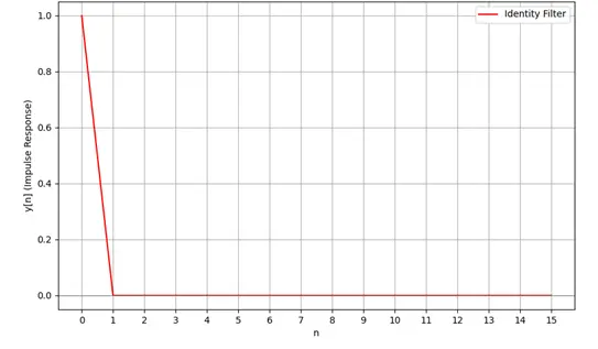
• x[n] is the current sample arriving right at that moment. So, the output is the same as input, i.e., 1 unit at n = 0 or, y[0] = 1 (Figure 1). This is also called an Identity Filter.

Figure 1: Output response from n = 0 to 15 units for the equation, y[n] = x[n]

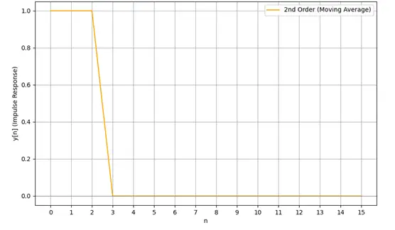
• x [n – 1] is the sample from one moment ago. With this, the output at n=1 also becomes 1 unit as the output is now the sum of current and one past input sample (Figure 2).

Figure 2: Output response for the equation, y[n] = x[n] + x[n-1]

• x [n – 2] is the sample from two moments ago. Adding this puts y [2] also at 1 unit since the output now depends on the sum of current input and two past inputs (Figure 3).

Figure 3: Output response for the equation, y[n] = x[n] + x[n-1] + x[n-2]

The b coefficients (b0, b1 and b2) function as weights for these input samples. The b0 decides how much of the current input signal is taken in the mix, while b1 and b2 decide the weightage of the past inputs that is to be included. Having more than one past input helps the filter to respond appropriately to immediate changes in the current input signal by averaging the recent input values.

Learning from Its Own History (The Feedback)

The second part of the equation, – a1 * y[n-1] – a2 * y[n-2], is where the filter gets its ability to remember and build upon its own past actions. This is the feedback part of the filter system as indicated by the subtraction.

• y [n – 1] is the output the filter produced one moment ago. This value allows us to smoothen the output response further, which now starts to represent a low-pass filter (Figure 4).

Figure 4: Output response for the equation with one past output sample feedback, y[n] = x[n] + x[n-1] + x[n-2] – 0.3 * y[n-1]

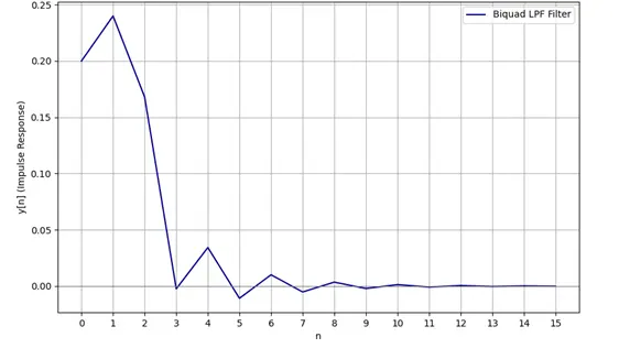
• y [n – 2] is the output from two moments ago. Inputting this in the equation now gives us a familiar low-pass filter which only passes values from y [0] to y [2] and blocks all values after that (Figure 5).

Figure 5: Output response for the equation, y[n] = x[n] + x[n-1] + x[n-2] – 0.3 * y[n-1] – 0.2 * y[n-2]

The coefficients a1 and a2, given by 0.3 and 0.2 here respectively, determine how much of these past outputs are fed back into the current calculation.

The Combined Effect in Digital Signal Processing

By setting these five “tuning knobs” (b0, b1, b2, a1 and a2), a biquad filter can dynamically transform any stream of numbers with near real-time speeds based on our design. It combines the samples for what is coming in right at that moment (current sample) with its memory of what just happened (past inputs) and what it last produced (past outputs) to allow users to effectively filter out any data from a stream of as per our requirement.

This simple, repetitive calculation, performed millions of times per second, is how digital filters achieve their remarkable ability to clean up, emphasize, or reshape signals.

The design and implementation of biquad filters are grounded in a well-established theory from digital signal processing and systems analysis.

Summary

The biquad filter is a remarkably efficient digital system that can intelligently weigh current and past inputs and dynamically learn from its own past outputs to process data the way we want to. Its power lies in how the five coefficients, like precision tuning knobs, can be adjusted to achieve incredibly diverse signal transformations.

However, this raises a fascinating question: How do engineers know what the exact values set for the a and b coefficients in the filter to create the low-pass filter? The answer to that lies in visualizing the filter’s “personality” on a powerful, intuitive map called the Z-plane.

At eInfochips, we leverage these fundamental DSP concepts to engineer robust and intelligent signal processing solutions to innovate ways of reliably interacting with the digital world around us.